Testing State Based Models#

This article explains how sinelaboreRT helps you test your state-based software.

In 2000 Martin Gomez wrote on embedded.com:

“The beauty of coding even simple algorithms as state machines is that the test plan almost writes itself. All you have to do is to go through every state transition. I usually do it with a highlighter in hand, crossing off the arrows on the state transition diagram as they successfully pass their tests. This is a good reason to avoid ‘hidden states’ - they’re more likely to escape testing than explicit states. Until you can use the ‘real’ hardware to induce state changes, either do it with a source-level debugger, or build an ‘input poker’ utility that lets you write the values of the inputs into your application.”

In many teams this is still common practice.

On a more general view state machine testing covers the following steps: (1) building a (test) model, (2) generating test cases (3) generating expected outputs, (4) running the tests, (5) comparing actual outputs with expected outputs, and (6) deciding on further actions (e.g. whether to modify the model, generate more tests, or stop testing).

Model based testing usually means that the test cases and other required data (e.g. test stimuli or expected test results) are derived automatically from the state machine model. And often also the automated test execution and validation is associated with model based testing. Probably only few organizations have implemented a fully automated test system covering all these steps. Especially for smaller teams the required investment for tools etc. is out of budget.

This article explains the features of sinelaboreRT that are relevant for (model based) testing. We use I) the Equivalent PCLopen function block and II) the microwave oven from the manual throughout this article. Both examples are available for download and allows you to follow all steps in. As we use the same model to generate code and testcases from step one is already done.

Generating test cases#

Defining testcases is the 2nd important step that usually consumes a lot of time if it must be done manually. The code generator can save you a lot of time by auto-matically suggesting test routes through a given state machine.

The used algorithm ensures that all transitions are taken at least once (100% transition coverage that also means 100% state coverage). So it is not anymore necessary to go through the diagram with a highlighter in hand. The following figure 1 shows the coverage information from the equivalent machine. The command line option ‘-c’ switches on the coverage data generation. The following command generates code and test routes from a Magic Draw model.

java -jar codegen.jar -v -c -p md -o equivalent -t "Model:Equivalent" equivalent.xml

The output looks the following:

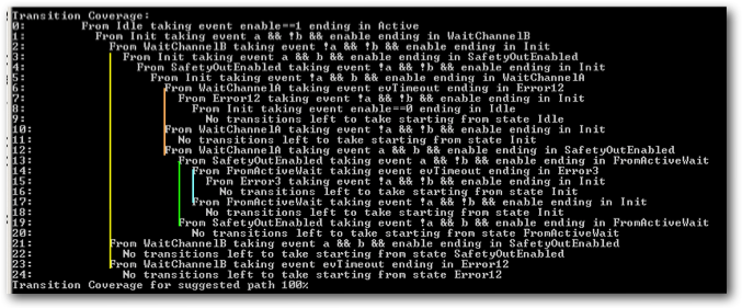
Automatic generation of test cases for 100 percent transition coverage

Figure 1: Coverage output generated from the code generator for the Safety Function Block state machine. The colored lines were added to better indicate the different routes.

You can see that the first test route starts from the initial state in line 0 and ends at line 9 where no untaken transitions are left to go (take a look in the state diagram below and follow the red arrows). The output moves to the right at every new transition on the route. Sometimes not all outgoing transitions of a state can be tested. In this case a branch in the test route is necessary. Take «WaitChannelB» as an example. As you can see not all transitions starting from WaitChannelB could be tested in one route. Two further branches are necessary. They are shown in line 21 and 23 (follow the yellow line) in figure 1. Branches are indicated by the same indentation level. Other branches in our example are marked with the red, green and blue lines.

SinelaboreRT can also generate an Excel sheet with all the test routes. More about this feature follows below.

State machine with test path

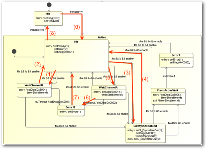
Figure 2: State machine with test path from step 0 to 8 as suggested from the coverage algorithm shown in figure 1.

Expected outputs#

To assess the test results the expected behavior must be defined. SinelaboreRT can not determine output values from the transitions or guards. It is your responsibility to define the output variables of the state machine (either hardware or software). But if you embed the expected output values in the state machine the code generator can extract it for you automatically.

To be able to extract the outputs you have to define it as so called state constraints. The UML does not directly support this so you have to define a comment and attach it to a state. In the comment use the ‘Constraints:’ key-word to start the constraints section. The format of the specification is up to you. An example for the ‘SafetyOutputState’ is shown in the following figure 3. In this case it is stated that the error output must be zero whereas the normal output must be one.

Use a comment to specify a constraint per state

Figure 3: Use a comment to specify a constraint per state.

Beside the console output from above - which provides a quick overview about the test effort - an Excel file can be created. It contains one route per sheet. Each line in a sheet is a single test step on the test route starting from the init state. There are as many sheets as routes are necessary to achieve the 100% transition coverage. A sheet lists the present state and the trigger to reach the next state. In addition the constraints of the source and the target states are listed. The constraint information is taken from the state diagram if specified (see figure 3 above). The following figure 4 shows the sheet for the state diagram from figure 2.

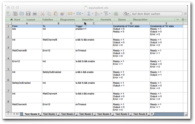Image that shows the test case in an Excel file Figure 4: Excel sheets with the test routes for the equivalent state machine. Each line contains a test step. If constraint data is provided in the state diagram (test oracle) it is added too. A tester can use this data as input for the test plan.

Running tests#

Test-beds are usually very hardware dependent in the embedded world. Therefore sinelaboreRT can’t generate a test-bed and the test case code for you. Using a unit test toolkit as described in [2] can be of great help here. To check that the machine is in the correct state you can instruct SinelaboreRT to generate trace code. Within the trace function you can send the trace data to a monitoring PC or store it e.g. for later analysis. This feature of SinelaboreRT is discussed in more detail in the second part of this article.

Comparing actual outputs and deciding on further actions#

Comparison of the actual outputs with expected outputs, and the decision on further actions (e.g. whether to modify the model, generate more tests, or stop testing) is a manual step. SinelaboreRT does not directly support this work.

Enabling tracing#

So far, we have shown how SinelaboreRT helps generate test cases to reach ideally 100% transition coverage. But SinelaboreRT can do more. You can connect your running target to an automatically generated visualization to show the current state of the state machine and possible triggers, all visually. It also shows the actually reached transition coverage.

We now use the microwave oven from the manual as an example. The code is available in the examples folder on GitHub.

The first step is to establish a link between the state machine running on the target and the SinelaboreRT visualization running on the PC. In this article, we assume that the state machine was created with the built-in editor. If you used another UML tool, convert your model file into the SinelaboreRT internal format by using -l ssc as the output format on the command line. The following example shows how to convert a CADIFRA model into the internal SCC representation:

java -jar codegen.jar -p CADIFRA -l ssc -o oven.xml oven.cdd

To generate trace code, use the -Trace command-line switch:

java -jar codegen.jar -c -Trace -p ssc -l cx -o oven oven.xml

You must provide the trace function yourself because it is typically system-dependent. Within this trace function, trace data can be sent to the monitoring PC. Because the function is under your control, you can use whatever hardware interface is practical for sending trace events. In most cases this will be a serial UART interface. If your target has TCP/IP capabilities, using UDP is recommended. The following code shows the trace function we use in this example.

void ovenTraceEvent(int evt){
    if (sendto(s,ovenTraceEvents[evt],
            strlen(ovenTraceEvents[evt]), 0,(const struct sockaddr *)&si_other,slen)==-1){
        perror("sendto\n");
        exit(1);
    }
}

Display the state diagram#

To display the state diagram, call the code generator with the -S command-line switch. A window, as shown in Figure 5, appears. The status of the state machine in its initial state is displayed.

java -jar codegen.jar -S -p ssc -o oven oven.xml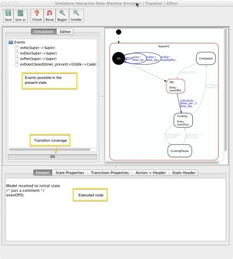

Microwave oven state machine visualization

Figure 5: The example shown here is the microwave oven state machine used in the manual. It is available in the examples folder of the SinelaboreRT download.

The main window shows the automatically generated state diagram. Events that can be handled at that moment are shown in blue. They are also listed in the left tree view. The output field at the bottom of the window shows the action code executed so far.

You can now send events to the machine by clicking on an event in the tree view. The display is updated accordingly and shows the new status.

To trace the real machine, we need a connection between the target and the visualization. For this reason, the code generator can receive events via UDP, as shown in the code snippet above. Most embedded systems do not offer an Ethernet connection directly. In this case, send trace data, for example, through a serial interface to the PC and forward it from there via UDP to the visualization. This can be implemented in just a few lines of code. This approach is used in the Asuro Mobile Robot example.

Testing at work#

Now we have prepared the visualization, so let us start the microwave oven example. To make this easy to follow, the microwave oven code was compiled as a simple console program. This program lets you set the cooking time and cooking power, and open and close the door using keyboard commands. When a cooking time is set and the door is closed, cooking starts. The console application prints debug messages, for example how much cooking time is left. When the time reaches zero, the microwave generator is switched off and the door must be opened before the next cooking cycle can start. The following figure shows this exact situation: cooking has ended. The current state is “Completed.” As you can see, only 57% transition coverage was reached during this test run.

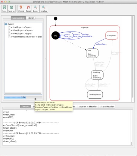
Transition coverage at 57 percent during test run

Figure 6: While testing, available transitions are displayed in blue and active states in red. The currently achieved transition coverage is shown as a progress bar below the event list.

Transitions not yet taken can be displayed as a tooltip on the progress bar. As you can see, we have not yet changed the cooking power or opened the door while cooking.

With this information at hand, it is easy to add the missing transitions to the test script and reach 100% transition coverage. Be aware that 100% transition coverage also means 100% state coverage.

So far, we have tested the device interactively, which in this case is the console application. To avoid this manual interaction (which is quite annoying for large machines), it is highly recommended to create a test environment that can be fed with test routes generated by the code generator (see the first part of this article series). This effort pays off quickly when extensions or bug fixes are needed and regression tests must be performed.

Testing not modeled behavior#

Even with 100% transition coverage you have only tested what was modeled. Often transitions that do not lead to a state change are omitted during the initial design. But from a testing point of view it is highly recommended to model such transitions too. Then the test route automatically include steps that check if the machine reacts correctly to transitions that do not change state!

Of course also perform boundary tests of used variables. For the microwave oven machine check for example what happens if the cooking time is zero and you still decrement it, or if it has reached its maximum and you still increment it etc. See the two recommended books listed in the Model-based testing of state diagrams of the article for many more practical hints.

Summary#

We close this article with citing again Martin Gomez who wrote “ … require a fair amount of patience and coffee, because even a mid-size state machine can have 100 different transitions. However, the number of transitions is an excellent measure of the system’s complexity. The complexity is driven by the user’s requirements: the state machine makes it blindingly obvious how much you have to test. With a less-organized approach, the amount of testing required might be equally large-you just won’t know it.”

This article has shown how sinelaboreRT helps you in testing your state based software. Therefore the different steps of testing were presented and how the sinelaboreRT code-generator supports you during the different test steps was discussed in detail.